This program is Copyright © 1976 by Hewlett-Packard and is used here by permission. This program was originally published in the HP-67 Standard Pac.
This program is supplied without representation or warranty of any kind. Hewlett-Packard Company and The Museum of HP Calculators therefore assume no responsibility and shall have no liability, consequential or otherwise, of any kind arising from the use of this program material or any part thereof.
| Curve Fitting | |||||
| Shift | P? | LIN? | EXP? | LOG? | PWR? |
| Label | xi↑yi(+) | xi↑yi(-) | →r2,a,b | y→x̂ | x→ŷ |
| Key | A | B | C | D | E |
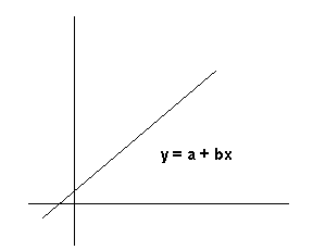
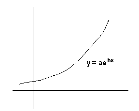
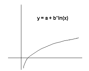
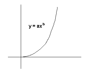
This program can be used to fit data to:
The type of curve fit must be determined before data input begins. To select linear regression, you would press the f B keys. To select exponential curve fit, press f C. To select logarithmic curve fit, press f D - To select power curve fit, press f E. Do not attempt to change from one type of fit to another after data input has begun because the summation registers are cleared when the type of curve fit is selected. Restarting can be accomplished by repeating the curve fit selection process.
Data pairs (xi and yi) are input by keying in xi, pressing ENTER↑ keying in yi and pressing the A key. Any number of data pairs may be input. If, after pressing the A key, you discover a data pair was incorrect, wait until execution stops, press h R↓ then the B key. This will eliminate the errant data pair. If you wish to eliminate any data pair previously input, key it in (x ENTER↑ y) and press B.
After all data pairs have been input, press C. This initiates calculation and output of the coefficient of determination r2, and the regression coefficients a and b. The coefficient of determination indicates the quality of fit achieved by the regression. Values of r2 close to 1.00 indicate a better fit than values close to zero. The regression coefficients a and b define the curve generated, according to the equations at the beginning of this discussion.
After the regression coefficients have been calculated, projections may be made based on the curve fit. Key in a known x value, press E and see an estimated y value, ŷ, or key in a known y value, press D and see an estimated x value, x̂.

     Σxiyi - (ΣxiΣyi)/n
b = ---------------------------
      Σxi2 - (Σxi)2/n

a = [Σyi/n - bΣxi/n]


         [Σxiyi - (Σxi*Σyi)/n]2
r2 = --------------------------------------------------
       [Σxi2 - (Σxi)2/n][Σyi2 - (Σyi)2/n]

     Σxi ln yi - (ΣxiΣ ln yi)/n
b = ------------------------------------
          Σxi2 - (Σxi)2/n

a = exp[(Σ ln yi)/n - b*(Σxi)/n]

          [Σxi ln yi - (ΣxiΣ ln yi)/n]2
r2 = --------------------------------------------------
      [Σxi2 - (Σxi)2/n][Σ(ln yi)2 - (Σ ln yi)2/n]

    Σyi*ln xi - (Σ ln xiΣyi)/n
b = -----------------------------
     Σ(ln xi)2 - (Σ ln xi)2/n

a = (Σyi - bΣ ln xi)/n

         [Σyi ln xi - Σ ln xiΣyi/n]2
r2 = --------------------------------------------------
      [Σ(ln xi)2 - (Σ ln xi)2/n][Σyi2-(Σyi)2/n]

     Σ(ln xi)(ln yi) - (Σ ln xi)(Σ ln yi)/n
b = -------------------------------------
         Σ(ln xi)2 - (Σ ln xi)2/n

a = exp[(Σ ln yi)/n - b(Σ ln xi)/n]

           [Σ(ln xi)(ln yi) - (Σ ln xi)(Σ ln yi)/n]2
r2 = -----------------------------------------------------
      [Σ(ln xi)2 - (Σ ln xi)2/n][Σ(ln yi)2 - (Σ ln yi)2/n]
Negative and zero values of xi will cause a machine error for logarithmic curve fits. Negative and zero values of yi will cause a machine error for exponential curve fits. For power curve fits both xi, and yi must be positive, non-zero values.
Registers R0-R9 are available for user storage.
It is not necessary to key in the x value if it corresponds to the counter returned to the display (see example 1).
As the differences between x and/or y values become small, the accuracy of the regression coefficients will decrease.
| Step | Instructions | Input Data/Units | Keys | Output Data/Units |
| 1 | Load side 1 and side 2. | |||
| 2 | Optional: Select pause input mode. | f A | 1.00 or 0.00 | |
| 3 | Select type of regression: | |||
| for linear fit | f B | 1.00 | ||
| for exponential fit | f C | 1.00 | ||
| for logarithmic fit | f D | 1.00 | ||
| for power fit | f E | 1.00 | ||
| 4 | Input x value*. | xi | ENTER↑ | xi |
| 5 | Input y value. | yi | A | i+1 |
| 6 | Repeat steps 4 and 5 for all data pairs**. | |||
| 7 | Compute and output coefficient of determination r2 and a and b. | C | r2, a, b | |
| 8 | Optional: Make projections based on a known y value. | y | D | est. x |
| 9 | Optional: Make projections based on a known x value. | x | E | est. y |
| 10 | For a new case go to step 3. | |||
| *Note that this step may be skipped if the x value equals the displayed counter (i + 1). | ||||
| **The last set of data pairs may be deleted by pressing h R↓ then B. Any set of data pairs may be deleted by entering them as in steps 4 and 5 and pressing B. |
Below is the sales data for the first 6 months of a product's life. According to a linear projection, what should the sales be after 12 months? When would sales reach the 150 unit per month mark assuming constant linear growth.
Month  1   2   3   4   5   6
Sales  15  37  52  59  83  92
Keystrokes                     Outputs
f B                              1.00
15 A 37 A 52 A 59 A 83 A 92 A    7.00
C                                0.98 *** (r2)
                                 3.33 *** (a)
                                15.14 *** (b)
12 E                           185.05     units
150 D                            9.69     months
The velocity of a particle experiencing constant acceleration is expressed by v = v0 + at where v is the velocity, v0 is the initial velocity, a is the acceleration and t is the time since v = v0.
The following data was experimentally obtained for a particle:
    t(sec)    V(m/sec)
      5         140
      6         149
      7         159
      9         175
What was the velocity at t = 0? What will the velocity be when t = 20? Note that the equation for velocity v = v0 + at is the equation of a straight line and is analogous to y = a + bx. Therefore use linear regression with v substituted for y, v0 for a, a (acceleration) for b and t for x.
Keystrokes                     Outputs
f B                             1.00
5 ENTER↑ 140 A 6 ENTER↑ 149 A
7 ENTER↑ 159 A                  4.00
9 ENTER↑ 175 A C                1.00 *** (r2)
                               96.54 *** (a, v0)
                                8.77 *** (b, acceleration)
20 E                          271.97 *** (m/sec)
Many compression processes can be correlated using the power curve p = av-b where b is the polytropic constant of the process.
Pressure-volume data for a compression process is shown below. Run a power curve fit to determine the polytropic constant, -b. What is the pressure when v is 15?
    v      p
   10     210
   30      40
   50      12
   70       9
   90       6.8
Keystrokes                     Outputs
f E                             1.00
10 ENTER↑ 210 A 30 ENTER↑ 40 A
50 ENTER↑ 12 A                  4.00
70 ENTER↑ 9 A 90 ENTER↑ 6.8 A
C                               0.99 *** (r2)
                             8599.81 *** (a)
                               -1.62 *** (-b)
15 E                          108.35
LINE  KEYS
001  *LBL a     Toggle print/pause mode flag.
002   0
003   F2?
004   RTN
005   1
006   SF 2
007   RTN
008  *LBL b     Clear flags and registers for linear
009   CF 0      regression.
010   CF 1
011   P⇔S
012   CL REG
013   P⇔S
014   1
015   RTN
016  *LBL c     Call LBL b, then set exponential flag.
017   GSB b
018   SF 1
019   RTN
020  *LBL d     Call LBL b, then set the logarithmic flag.
021   GSB b
022   SF 0
023   RTN
024  *LBL e     Call LBL d, then set the power curve flag.
025   GSB d
026   SF 1
027   RTN
028  *LBL A     Clear Σ- flag.
029   CF 3
030  *LBL 8
031   F2?       Print if flag 2 is set.
032   GSB 9
033   STO D
034   F1?       ln y if flag 1 is set.
035   LN
036   X⇔Y       ln x if flag 0 is set.
037   STO C
038   F0?
039   LN
040   F3?       If flag 3, then Σ-.
041   GTO 0
042   Σ+        Compute sums.
043  *LBL 7     Calculate i + 1.
044   ENTER↑
045   1
046   +
047   RCL C     Set inputs in stack positioned for possible
048   X⇔Y       deletion.
049   RCL D
050   X⇔Y
051   RTN
052  *LBL 0     Subtract from sums.
053   Σ-
054   GTO 7
055  *LBL 9     Print inputs and reset print flag.
056   PRT SPC
057   X⇔Y
058   PRTX
059   X⇔Y
060   PRTX
061   SF 2
062   RTN
063  *LBL B
064   SF 3      Set Σ- flag.
065   F2?       Print delete indicator if flag is set.
066   GSB 3
067   GTO 8     Delete inputs.
068  *LBL C     Switch to secondary registers.
069   P⇔S
070   PRT SPC   Compute b.
071   RCL 8
072   RCL 4
073   RCL 6
074   ×
075   RCL 9
076   ÷
077   -
078   ENTER↑
079   ENTER↑
080   RCL 4
081   x2
082   RCL 9
083   ÷
084   RCL 5
085   X⇔Y
086   -
087   ÷
088   STO B
089   ×         Compute r2.
090   RCL 6
091   x2
092   RCL 9
093   ÷
094   CHS
095   RCL 7
096   +
097   ÷
098   PRTX
099   RCL 6     Compute a.
100   RCL 4
101   RCL B
102   ×
103   -
104   RCL 9
105   ÷
106   F1?
107   eX
108   STO A
109   PRTX      Output a and b.
110   RCL B
111   PRTX
112   P⇔S       Switch registers.
113   RTN
114  *LBL E     Position coefficients in stack for use by
115   STO E     projection routines.
116   RCL A
117   RCL B
118   RCL E
119   F1?       If flag 1 is set, power or exponential
120   GTO 1     projection.
121   F0?
122   LN        Logarithmic?
123   ×
124   +         Linear or logarithmic projection.
125   F2?
126   GTO 9     Print?
127   RTN       Stop
128  *LBL 1
129   F0?       If flag 0 is set, do power fit.
130   GTO 2
131   ×         Do exponential projection.
132   eX
133   ×
134   F2?       Print?
135   GTO 9
136   RTN       Stop
137  *LBL 2
138   X⇔Y
139   Yx        Do power projection.
140   ×
141   F2?       Print?
142   GTO 9
143   RTN       Stop
144  *LBL 3
145   PRT SPC   Print -1 indicator.
146   1
147   CHS
148   PRTX
149   SF 2
150   R↓
151   RTN
152  *LBL D     Position coefficients in stack for use by
153   STO E     projection routine.
154   RCL B
155   1/X
156   RCL A
157   RCL E
158   X⇔Y
159   F1?
160   GTO 1     Power or exp?
161   -
162   ×         Linear and log projection.
163   F0?
164   ex        Logarithmic.
165   F2?       Print?
166   GTO 9
167   RTN       Stop
168  *LBL 1
169   ÷         Calculate exp calc.
170   F0?       For power, GTO 1
171   GTO 1
172   LN        Exponential projection.
173   ×
174   F2?
175   GTO 9     Print?
176   RTN       Stop
177  *LBL 1
178   X⇔Y       Power projection.
179   YX
180   F2?       Print?
181   GTO 9
182   RTN       Stop
183   R/S
S0  0
S1  0
S2  0
S3  0
S4  Σx
S5  Σx2
S6  Σy
S7  Σy2
S8  Σxy
S9  n
A   a
B   b
C   xi
D   yi
E   x,y
I   0
![]() Go back to the software library
Go back to the software library
![]() Go back to the main exhibit hall
Go back to the main exhibit hall